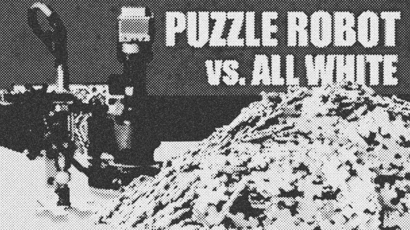
Solving the Impossible: Algorithmically Assembling a 4,000-Piece All-White Puzzle

Solving an all-white puzzle is the ultimate hardware and software stress test. Without visual cues or image features, you are left with nothing but geometry. A 4,000-piece puzzle requires approximately 30 million physical comparisons if approached manually—a task that would take a human years. This tutorial breaks down the computer vision and algorithmic techniques required to automate this process, moving from raw pixel data to a fully realized

(LSH) system for high-speed geometric matching.

Prerequisites

To implement these concepts, you should be comfortable with:

• Python: The primary language for prototyping computer vision logic.
• Image Processing: Understanding thresholding and pixel-to-contour conversion.
• Geometry: Familiarity with polygons and curve fitting.
• Data Structures: Specifically hashes and multi-dimensional coordinate systems.

Key Libraries & Tools

• OpenCV: Used for initial image acquisition and extracting the contour (edge) of the puzzle pieces.
• NumPy: Essential for handling the 128-dimensional arrays used in the hashing phase.
• Puget Systems Workstations: High-performance hardware used to parallelize the pre-processing tasks.
• Telecentric Lens: A critical piece of optics that eliminates perspective distortion, ensuring the puzzle piece dimensions remain accurate across the frame.

Code Walkthrough: From Pixels to Hashing

1. Shape Extraction and Edge Normalization

First, we isolate the puzzle piece from the background using thresholding. Once we have a binary blob, we identify the perimeter and convert it into a polygon. The real challenge is finding the corners to split the perimeter into four distinct edges.

# Conceptual approach for finding clean corners
for corner in approximate_corners:
    # Grab small segments of the polygon on either side of the corner
    curve_a = fit_curve(polygon_segment_left)
    curve_b = fit_curve(polygon_segment_right)
    
    # The intersection of these curves is the 'true' geometric corner
    true_corner = intersect(curve_a, curve_b)
    
    # Split the polygon at the point closest to this intersection
    split_point = find_closest_point(polygon, true_corner)

2. Locality-Sensitive Hashing (LSH)

To avoid comparing every edge to every other edge (an $O(n^2)$ nightmare), we use

. We project 128-dimensional edge features into a hashed sequence. Similar shapes fall into the same "bucket," allowing for $O(1)$ lookup.

# 128-dimensional projection (Simplified logic)
def get_lsh_hash(edge_points, hyperplanes):
    # edge_points is a vector approximating the curve shape
    # hyperplanes define the boundaries in high-dimensional space
    hash_sequence = ""
    for plane in hyperplanes:
        if dot_product(edge_points, plane) > 0:
            hash_sequence += "1"
        else:
            hash_sequence += "0"
    return hash_sequence

Syntax Notes: High-Dimensional Space

While we visualize geometry in 2D or 3D, the algorithm uses a 128-dimensional space. In this context, a "line" becomes a hyperplane. The syntax for determining which side of a hyperplane a point falls on is a simple dot product. This mathematical efficiency is what allows the robot to identify potential matches in milliseconds rather than hours.

Practical Examples: Hierarchical Assembly

Once potential matches are identified, the software doesn't just guess. It employs a recursive block-building strategy. It finds valid 2x2 blocks by ensuring pieces share mutual neighbors. These 2x2 blocks are then treated as "super-pieces" to form 4x4 blocks, continuing until the entire grid is solved. This dramatically reduces the search space by eliminating local geometric matches that don't fit the global grid.

Tips & Gotchas

• Garbage In, Garbage Out: If your puzzle pieces have fuzzy edges from a dull die-cutter, your algorithm will fail. Use a laser cutter or a vibratory tumbler to ensure sharp, clean edges.
• Pre-processing Latency: Extracting 4,000 piece shapes can take days. Use Python's multiprocessing to split the job into smaller tasks across all available CPU cores.
• Cumulative Error: In physical assembly, small misalignments add up. Your robot needs a secondary camera to "nudge" pieces into place as the grid grows.